Stanford Simbios group
Back to NA-MIC External Collaborations
Grant#
- U54EB005149-05S2
Key Personnel
- Stanford Simbios (U54LM008748): Scott Delp, PI, Harris Doddi, Saikat Pal
- NA-MIC: Ron Kikinis, Steve Pieper
- Kitware: Luis Ibanez
Grant Duration
09/19/2008-07/31/2010


Aims
The purpose of this project is to develop a methodology to rapidly construct three-dimensional anatomical structures from magnetic resonance (MR) imaging for clinical diagnosis. We are currently interested in segmenting hip bone geometry of patients prior to femoral acetabular impingement surgery. The clinical motivation for this study is to eliminate the need for computed tomography (CT) scanning and associated radiation dose in patients during surgical planning.
The specific aims are -
Aim 1: Develop a software pipeline to rapidly segment hip bone geometry from MR data.
Aim 2: Evaluate the accuracy of the proposed MR-based segmentation method with models segmented from computer tomography (CT) scanning.
Process Flowchart
The pipeline shows the steps required for segmentation of hip joint structures. The steps in red represent user interactions.

Progress
Update June 05, 2010


Recent work:
1. We optimized an MR protocol to maximize signal-to-noise ratio of the pelvic region imaging with a cardiac body coil. We experimented with different scan sequences and found an IDEAL SPGR sequence to provide the best contrast for our application. We imaged 6 healthy subjects to acquire their IDEAL SPGR fat and water images. The total scan time per subject is about 20 minutes.
2. We implemented a semi-automatic segmentation pipeline using a combination of ITK filters and custom scripting. The inputs to the pipeline were IDEAL SPGR Fat and Water MR images. The outputs were 3D outlines of regions-of-interest.
Next steps:
1. Currently, we are able to extract the hip joint structures that closely match MR data with minimal user interaction. However, to improve the accuracy of our segmentation, we are implementing a manual refinement step. Using a GUI-based interface, a user will be able to improve on the output of the modeling pipeline.
2. Evaluate the accuracy of our MR-based segmentation with geometry acquired from CT imaging. We will quantify the accuracy of our method by calculating the percentage difference in enclosed volumes between MR- and CT-based geometries.
Atlas Generation from Input MR Images
Model Generation from Input MR Images
Pre-Segmented models for femur, patella and tibia are obtained for a patient (in .stl format).
Create a filled label map using PolyDataToFilledLabelMap module in slicer
The models generated in the above step are closed but hollow. But EM Segmentation requires the atlas given to be in closed filled format. Hence we converted the hollow closed models into filled label volumes using the module PolyDataToFilledLabelMap module in Slicer. The output label map of this module is of datatype unsigned char and is converted to short datatype.


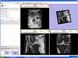
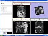
EM Segmentation based on the atlas
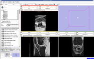
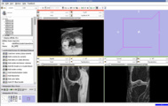
The output label map in the above is given as input atlas in the EM Segmentation step. As an initial step we ran EM Segmentation on the same patient. The EM Segmented output is given in the below figure.
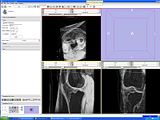
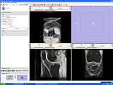
Register Images
Register Images Module in Slicer
We are now in the process of trying to register new patient image to the existing patient image. If we register the images, we can get the transform which can be used to register the existing atlas (label map) to the new patient.
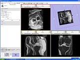
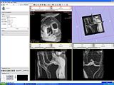
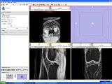
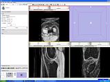
We think that Pipelined Bspline Registration may give promising results for our dataset. Below are some of the results. Here we consider 64_MRI as the fixed image and 58_MRI as the moving image and used Pipelined BSpline Image registration method for registration. Also we gave one point as landmark point.


We also tried affine registration for the above mentioned patients with 64 as fixed MRI and 58 as moving MRI and one landmark point. The zipped file which contains scene along with screenshots is File:64 58 Affine Registration.zip


We also tried BSpline registration for the above mentioned patients with 64 as fixed MRI and 58 as moving MRI and one landmark point. The zipped file which contains scene along with screenshots is
File:64 58 BSpline Registration.zip. Here we used 4 points as landmarks.


We also tried Affine registration for the above mentioned patients with 64 as fixed MRI and 58 as moving MRI and four landmark point. The zipped file which contains scene along with screenshots is
File:64 58 Affine Various Iterations.zip. Here we used 4 points as landmarks. We varied the number of iterations from 200 to 400.


Update May 13, 2009
We tried Affine registration for the above mentioned patients with 64 as fixed MRI and 58 as moving MRI and no landmark point. The zipped file which contains scene along with screenshots is File:64 58 Affine Various Iterations.zip. We varied the number of iterations from 200 to 400.
Update May 14, 2009
We tried Affine registration for the above mentioned patients with 64 as fixed MRI and 58 as moving MRI and 10 landmark point. The zipped file which contains scene along with screenshots is File:Affine Registration 10 Landmark Points Varying Iterations.zip. We varied the number of iterations from 50 to 450.


- 64 58 Affine 450 Iterations 10 Landmark Points.jpg


Update May 20, 2009
We tried BSpline registration for the above mentioned patients with 64 as fixed MRI and 58 as moving MRI and no landmark point. The zipped file which contains scene along with screenshots is File:Affine Registration 10 Landmark Points Varying Iterations.zip. We varied the number of iterations from 50 to 450.

- 64 58 BSpline 360 Iterations.JPG


Update May 21, 2009
We tried Pipelined Affine registration for the above mentioned patients with 64 as fixed MRI and 58 as moving MRI and no landmark point. The zipped file which contains scene along with screenshots is File:BSpline Registration Varying Iterations.zip. We varied the number of iterations from 50 to 450.

- 64 58 PipeLinedAffine Registration 400 Iterations.JPG


Update May 25, 2009
We tried Affine registration for the above mentioned patients with 64 as fixed MRI and 58 as moving MRI and no landmark point. The zipped file which contains scene along with screenshots is File:BSpline Registration Varying Iterations.zip. We varied the number of iterations from 50 to 5000.


Multi Image Registration
We have also tried the approach of Non-rigid Groupwise Registration using Bspline Deformation Model by Serdar K. Balci, Polina Golland and William M. Wells. In this approach, we try to give one slice each of two different patients we need to register as input. Here are some of the results of their approach.
- Slice 1:
- Slice 2:
- Mean Slice of above two :


- Slice 1:
- Slice 2:
- Mean Slice of above two :
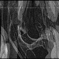


Image Segmentation Methods (Oct-Dec) 2009
Shape Dectection Level Set Approach
We started in October with Shape Dectection Level Set algorithm. In this algorithm, the governing differential equation has an additional curvature-based term. This term acts as a smoothing term where areas of high curvature, assumed to be due to noise, are smoothed out. Scaling parameters are used to control the tradeoff between the expansion term and the smoothing term. One consequence of this additional curvature term is that the fast marching algorithm is no longer applicable, because the contour is no longer guaranteed to always be expanding. Instead, the level set function is updated iteratively. The ShapeDetectionLevelSetImageFilter expects two inputs, the first being an initial Level Set in the form of an itk::Image, and the second being a feature image. For this algorithm, the feature image is an edge potential image that basically follows the same rules applicable to the speed image used for the FastMarchingImageFilter. The pipeline of the algorithm is as follows

The output of this algorithm is as follows.


The models extracted from the segmented label maps are as follows.


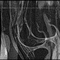
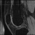
Multi-Contrast MR Approach
In this algorithm, we try to collect MR images of Knee using different MR scans like IDEAL-SPGR-FAT, IDEAL-SPGR-WATER, IDEAL-GRE-FAT etc. The main assumption in this algorithm is that different structures of interest ( eg: bones/cartilage) have different intensity values in different scans. For eg: Bones are colored with lower pixel intensity values in IDEAL-SPGR-WATER dataset whereas they are colored with higher pixel intensity values in IDEAL-SPGR-WATER dataset.
Firstly, we collect the seed points of the regions of interest using an insight application "ImageViewer". So each file with the seed points is considered as one cluster. For eg: we can have clusters for background, bones, cartilage etc. Next, we calculate the cluster centers (µ) and standard deviation (ρ) for each seed file. We try to define user defined parameter called numberOfSd(α) which represents the extent of how far a cluster can go. The numberofSd(α) has been split to be bi-directional in the x-axis representing one contrast image and y-axis representing another contrast image.
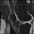
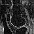
Below is the dataset of Knee MR image we used
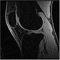
IDEAL-SPGR-WATER
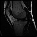
IDEAL-SPGR-FAT


Scatter Plot of the above two images
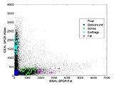
Scatter Plot

Segmentation Output we obtained :
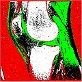
Red: Background

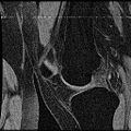
We have also proved that our algorithm works fairly well for hip dataset. Below are the MR images of Hip dataset we used.


The segmented output we got using our approach is

Datasets
1. IDEAL-SPGR-FAT dataset File:IdealSPGRFat.zip
2. IDEAL-SPGR-WATER dataset File:IdealSPGRWater.zip
Future Work
Build Models from the segmented label maps that we get from Multi MR contrast images.
Extend our existing Multi Contrast MR solution to other body datasets.
Improve segmentation results from our current dataset by using "more" multi contrast images.
References
1. ITK Software Guide ( http://www.itk.org)
2. Slicer Software (http://www.slicer.org)
3. Multi-Contrast MR for Enhanced Bone Imaging and Segmentation Ruphin Dalvi, Rafeef Abugharbieh, Derek C. Wilson, David R. Wilson.
4. HE Cline. WE Lorensen, R Kikinis, F Jolesz 3D Segmentation of the Head Using Probability and Connectivity Journal of Computer Assisted Tomography 14:1037-1045 (1990)