Difference between revisions of "Projects:GroupwiseRegistration"
| (41 intermediate revisions by 7 users not shown) | |||
| Line 1: | Line 1: | ||
| − | Back to [[NA- | + | Back to [[NA-MIC_Internal_Collaborations:StructuralImageAnalysis|NA-MIC Collaborations]], [[Algorithm:MIT|MIT Algorithms]] |
| − | + | __NOTOC__ | |
= Non-rigid Groupwise Registration = | = Non-rigid Groupwise Registration = | ||
| Line 25: | Line 25: | ||
| − | + | ''Objective Function'' | |
| − | |||
| − | |||
| − | |||
[[Image:GroupwiseStackBiModal.PNG|thumb|350px|Figure 1: On the left is shown a stack of images | [[Image:GroupwiseStackBiModal.PNG|thumb|350px|Figure 1: On the left is shown a stack of images | ||
| Line 50: | Line 47: | ||
| − | + | ''Deformation Model'' | |
| + | |||
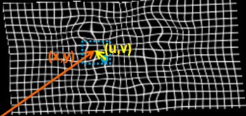
| + | [[Image:GroupwiseBspline.png|thumb|350px|Figure 2: An example deformation field. The local neighborhood affecting the deformation is overlayed on the image.]] | ||
For the nonrigid deformation model, | For the nonrigid deformation model, | ||
| Line 70: | Line 69: | ||
</math> | </math> | ||
| − | + | ||
| − | where | + | where <math>B_l</math> is <math>l</math>'th cubic B-spline basis function. <math>(u,v,w)</math> is the distance |
to <math>(x,y,z)</math> from the control point <math>\Phi_{i,j,k}</math> as shown in Figure 2. | to <math>(x,y,z)</math> from the control point <math>\Phi_{i,j,k}</math> as shown in Figure 2. | ||
| Line 79: | Line 78: | ||
| − | + | ''Implementation'' | |
| − | |||
| − | |||
| − | |||
| − | |||
| − | |||
| − | |||
| − | |||
| − | |||
| − | |||
| − | |||
| − | |||
| − | |||
| − | |||
| − | + | [[Image:GroupwiseIncreasingScale.PNG|thumb|350px|Figure 3: A registration schedule using gradually increasing deformation field complexity. From left to right deformation fields for increasing deformation field complexity. ]] | |
| − | |||
| − | |||
| − | |||
| − | |||
| − | |||
| − | |||
| − | |||
| − | |||
| − | |||
| − | |||
| − | to | ||
| − | |||
| − | |||
| − | |||
| − | |||
| − | |||
| − | |||
| − | |||
| − | |||
We provide an efficient optimization scheme by using line search with the gradient descent algorithm. | We provide an efficient optimization scheme by using line search with the gradient descent algorithm. | ||
| − | For computational efficiency, we employ a stochastic subsampling procedure | + | For computational efficiency, we employ a stochastic subsampling procedure. |
In each iteration of the algorithm, | In each iteration of the algorithm, | ||
a random subset is drawn from all samples and the objective function is evaluated | a random subset is drawn from all samples and the objective function is evaluated | ||
only on this sample set. | only on this sample set. | ||
| − | |||
| − | |||
| − | |||
To obtain a dense deformation field capturing anatomical variations at different scales, | To obtain a dense deformation field capturing anatomical variations at different scales, | ||
we gradually increase the complexity of the deformation field by refining the grid of B-spline control points. | we gradually increase the complexity of the deformation field by refining the grid of B-spline control points. | ||
| − | + | ||
| − | + | ||
| − | + | [[Image:GroupwiseMultiResolution.PNG|thumb|350px|Figure 4: An example showing the multi-resolution scheme. The registration is first performed at a coarse scale by downsampling the input. | |
| − | + | Results from coarser scales are used to initialize | |
| − | + | optimization at finer scales. Also note that the objective function is only evaluated on a small subset of input points. ]] | |
As in every iterative search algorithm, local minima pose a significant problem. | As in every iterative search algorithm, local minima pose a significant problem. | ||
To avoid local minima we use a multi-resolution optimization scheme for each resolution level of the deformation field. | To avoid local minima we use a multi-resolution optimization scheme for each resolution level of the deformation field. | ||
| − | |||
| − | |||
| − | |||
| − | |||
| − | |||
| − | We implemented our groupwise registration method in a multi-threaded fashion using Insight Toolkit (ITK) | + | We implemented our groupwise registration method in a multi-threaded fashion using Insight Toolkit(ITK) |
| − | and made the implementation publicly available | + | and made the implementation publicly available [http://www.na-mic.org/svn/NAMICSandBox/trunk/MultiImageRegistration/ (code)]. |
| − | |||
| − | |||
| − | |||
| − | |||
| − | |||
| − | |||
| + | ''Results'' | ||
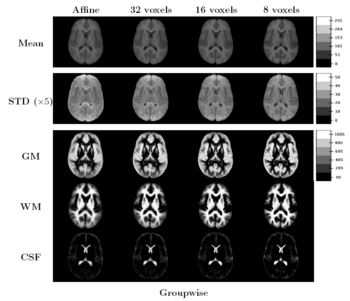
| + | [[Image:GroupwiseMeanImages.png|thumb|350px|Figure 5: Central slices of 3D volumes for groupwise registration. Rows show mean and standard deviation images followed by label overlap images for GM, WM and CSF labels. Columns display the results for affine and B-splines with grid spacing 32, 16 and 8 voxels, respectively. ]] | ||
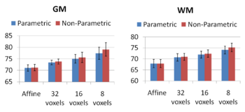
| + | [[Image:GroupwiseBarsWMGM.png|thumb|350px|Figure 6: GM, WM DICE measures computed for different deformation field resolution levels. Blue bars show the results for groupwise registration and the red bars show the results for registration to the mean setting.]] | ||
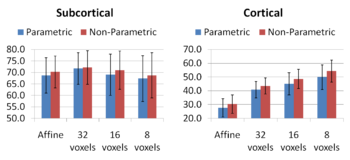
| + | [[Image:GroupwiseBarsManual.png|thumb|350px|Figure 7: DICE measures for manually segmented labels. Bars correspond to the same setting as in figure 6. ]] | ||
| − | |||
| − | We tested the groupwise registration algorithm on a MR brain dataset | + | We tested the groupwise registration algorithm on a MR brain dataset. |
| − | |||
The dataset consists of 50 MR brain images of three subgroups: | The dataset consists of 50 MR brain images of three subgroups: | ||
schizophrenics, affected disorder and normal control patients. | schizophrenics, affected disorder and normal control patients. | ||
| − | MR images are T1 scans with | + | MR images are T1 scans with 256x256x128 voxels |
| − | and | + | and 0.9375x0.9375x1.5 mm<sup>3</sup> spacing. |
| − | + | For each image in the dataset, an automatic tissue classification | |
| − | |||
| − | |||
| − | For each image in the dataset, an automatic tissue classification | ||
was performed, yielding gray matter (GM), white matter (WM) and cerebro-spinal | was performed, yielding gray matter (GM), white matter (WM) and cerebro-spinal | ||
fluid (CSF) labels. In addition, manual segmentations of four subcortical regions | fluid (CSF) labels. In addition, manual segmentations of four subcortical regions | ||
| Line 168: | Line 120: | ||
gyrus and para-hippocampus) were available for each MR image. | gyrus and para-hippocampus) were available for each MR image. | ||
| − | |||
| − | |||
| − | |||
| − | |||
| − | |||
| − | |||
| − | |||
| − | |||
Increasing the complexity of the deformation model improves the | Increasing the complexity of the deformation model improves the | ||
accuracy of prediction. An interesting open problem is automatically | accuracy of prediction. An interesting open problem is automatically | ||
| Line 195: | Line 139: | ||
Comparing the groupwise registration to the pairwise approach, we | Comparing the groupwise registration to the pairwise approach, we | ||
observe that the sharpness of the mean images and the tissue overlaps | observe that the sharpness of the mean images and the tissue overlaps | ||
| − | in Figure | + | in Figure 5 look visually similar. From Figures 6 and 7, we note that |
groupwise registration performs slightly better than the pairwise | groupwise registration performs slightly better than the pairwise | ||
setting in most of the cases, especially as we increase the complexity | setting in most of the cases, especially as we increase the complexity | ||
| Line 203: | Line 147: | ||
image. However, the advantage shown here is only slight; more | image. However, the advantage shown here is only slight; more | ||
comparative studies are needed of the two approaches. | comparative studies are needed of the two approaches. | ||
| − | |||
| − | |||
| − | |||
| − | |||
| − | |||
| − | |||
| − | |||
| − | |||
| − | |||
| − | |||
| − | |||
| − | |||
| − | |||
| − | |||
| − | |||
| − | |||
| − | |||
| − | |||
| − | |||
| − | |||
| − | |||
| − | |||
| − | |||
| − | |||
| − | |||
| − | |||
| − | |||
| − | |||
| − | |||
| − | |||
| − | |||
| − | |||
| − | |||
| − | |||
| − | |||
| − | |||
| − | |||
| − | |||
| − | |||
We compare our groupwise algorithm to a pairwise method where we register | We compare our groupwise algorithm to a pairwise method where we register | ||
each subject to the mean intensity using sum of square differences. | each subject to the mean intensity using sum of square differences. | ||
| − | |||
| − | |||
| − | |||
| − | |||
| − | |||
During each iteration we consider the mean image as a reference image | During each iteration we consider the mean image as a reference image | ||
and register | and register | ||
| Line 255: | Line 155: | ||
After each iteration the mean image is updated and pairwise registrations are performed until convergence. | After each iteration the mean image is updated and pairwise registrations are performed until convergence. | ||
| − | + | The images in Figure 5 show central slices of 3D images after registration. | |
| − | |||
| − | The images in Figure | ||
Visually, mean images get sharper and variance images becomes darker, especially around central ventricles and cortical regions. | Visually, mean images get sharper and variance images becomes darker, especially around central ventricles and cortical regions. | ||
We can observe that anatomical variability at cortical regions causes significant blur for | We can observe that anatomical variability at cortical regions causes significant blur for | ||
| Line 264: | Line 162: | ||
the tissue label overlap images get sharper. | the tissue label overlap images get sharper. | ||
| + | =Asymmetric Image-Template Registration= | ||
| − | + | A natural requirement in pairwise image registration is that the resulting deformation is independent of the order of the images. This constraint is typically achieved via a symmetric cost function and has been shown to reduce the effects of local optima. Consequently, symmetric registration has been successfully applied to pairwise image registration as well as the spatial alignment of individual images with a template. However, recent work has shown that the relationship between | |
| − | + | an image and a template is fundamentally asymmetric. In this work, we develop a method that reconciles the practical advantages of symmetric registration with the asymmetric nature of image-template registration by adding a simple correction factor to the symmetric cost function. We instantiate our model within a log-domain diffeomorphic registration | |
| − | + | framework. Our experiments show exploiting the asymmetry in image-template registration improves alignment in the image coordinates. | |
| − | |||
| − | |||
| − | |||
| − | |||
| − | |||
| − | |||
| − | |||
| − | |||
| − | |||
| − | |||
| − | |||
| − | |||
| − | |||
= Key Investigators = | = Key Investigators = | ||
| − | * | + | * MIT: Mert R. Sabuncu, B.T. Thomas Yeo, Koen Van Leemput, Serdar K. Balci, Polina Golland. |
| + | * Harvard: Sylvain Bouix, Martha E. Shenton, Bruce Fischl, W.M. (Sandy) Wells. | ||
| + | * Kitware: Brad Davis, Louis Ibanez. | ||
= Publications = | = Publications = | ||
| − | + | ||
| + | [http://www.na-mic.org/publications/pages/display?search=Projects%3AGroupwiseRegistration&submit=Search&words=all&title=checked&keywords=checked&authors=checked&abstract=checked&sponsors=checked&searchbytag=checked| NA-MIC Publications Database on Groupwise Registration] | ||
| + | |||
| + | [[Category: Registration]] [[Category:Segmentation]] [[Category:MRI]] [[Category:Schizophrenia]] | ||
Latest revision as of 20:07, 11 May 2010
Home < Projects:GroupwiseRegistrationBack to NA-MIC Collaborations, MIT Algorithms
Non-rigid Groupwise Registration
We aim at providing efficient groupwise registration algorithms for population analysis of anatomical structures. Here we extend a previously demonstrated entropy based groupwise registration method to include a free-form deformation model based on B-splines. We provide an efficient implementation using stochastic gradient descents in a multi-resolution setting. We demonstrate the method in application to a set of 50 MRI brain scans and compare the results to a pairwise approach using segmentation labels to evaluate the quality of alignment. Our results indicate that increasing the complexity of the deformation model improves registration accuracy significantly, especially at cortical regions.
Description
We first describe the stack entropy cost function and the B-spline based deformation model. Then we discuss implementation details. Next, we compare groupwise registration to the pairwise method and evaluate both methods using label prediction values.
Objective Function

In order to align all subjects in the population, we consider sum of pixelwise entropies as a joint alignment criterion. The justification for this approach is that if the images are aligned properly, intensity values at corresponding coordinate locations from all the images will form a low entropy distribution. This approach does not require the use of a reference subject; all subjects are simultenously driven to the common tendency of the population.
We employ a kernel based density estimation scheme to estimate univariate entropies. Using the entropy measure we obtain a better treatment of transitions between different tissue types, such as gray matter-white matter transitions in the cortical regions where intensity distributions can be bi-modal as shown in Figure 1.
Deformation Model
For the nonrigid deformation model, we define a combined transformation consisting of a global and a local component
- [math] T(\mathbf{x}) = T_{local}({T_{global}(\mathbf{x})}) [/math]
where [math]T_{global}[/math] is a twelve parameter affine transform and [math]T_{local}[/math] is a deformation model based on B-splines.
The free form deformation can be written as the 3-D tensor product of 1-D cubic B-splines.
- [math] T_{local}(\mathbf{x}) = \mathbf{x} + \sum_{l=0}^3\sum_{m=0}^3\sum_{n=0}^3 B_l(u)B_m(v)B_n(w) \Phi_{i+l,j+m,k+n} [/math]
where [math]B_l[/math] is [math]l[/math]'th cubic B-spline basis function. [math](u,v,w)[/math] is the distance to [math](x,y,z)[/math] from the control point [math]\Phi_{i,j,k}[/math] as shown in Figure 2.
The deformation of a given point can be found using only the control points in the neighborhood of the given point. Therefore, optimization of the objective function can be implemented efficiently.
Implementation
We provide an efficient optimization scheme by using line search with the gradient descent algorithm. For computational efficiency, we employ a stochastic subsampling procedure. In each iteration of the algorithm, a random subset is drawn from all samples and the objective function is evaluated only on this sample set.
To obtain a dense deformation field capturing anatomical variations at different scales, we gradually increase the complexity of the deformation field by refining the grid of B-spline control points.

As in every iterative search algorithm, local minima pose a significant problem. To avoid local minima we use a multi-resolution optimization scheme for each resolution level of the deformation field.
We implemented our groupwise registration method in a multi-threaded fashion using Insight Toolkit(ITK) and made the implementation publicly available (code).
Results
We tested the groupwise registration algorithm on a MR brain dataset.
The dataset consists of 50 MR brain images of three subgroups:
schizophrenics, affected disorder and normal control patients.
MR images are T1 scans with 256x256x128 voxels
and 0.9375x0.9375x1.5 mm3 spacing.
For each image in the dataset, an automatic tissue classification
was performed, yielding gray matter (GM), white matter (WM) and cerebro-spinal
fluid (CSF) labels. In addition, manual segmentations of four subcortical regions
(left and right hippocampus and amygdala) and four cortical regions (left and right superior temporal
gyrus and para-hippocampus) were available for each MR image.
Increasing the complexity of the deformation model improves the accuracy of prediction. An interesting open problem is automatically identifying the appropriate deformation complexity before the registration overfits and the accuracy of prediction goes down. We also note that the alignment of the subcortical structures is much better than that of the cortical regions. It is not surprising as the registration algorithm does not use the information about geometry of the cortex to optimize the alignment of the cortex. In addition, it has been often observed that the cortical structures exhibit higher variability across subjects when considered in the 3D volume rather than modelled on the surface.
Our experiments highlight the need for further research in developing evaluation criteria for image alignment. We used the standard Dice measure, but it is not clear that this measurement captures all the nuances of the resulting alignment.
Comparing the groupwise registration to the pairwise approach, we observe that the sharpness of the mean images and the tissue overlaps in Figure 5 look visually similar. From Figures 6 and 7, we note that groupwise registration performs slightly better than the pairwise setting in most of the cases, especially as we increase the complexity of the warp. This suggests that considering the population as a whole and registering subjects jointly brings the population into better alignment than matching each subject to a mean template image. However, the advantage shown here is only slight; more comparative studies are needed of the two approaches.
We compare our groupwise algorithm to a pairwise method where we register each subject to the mean intensity using sum of square differences. During each iteration we consider the mean image as a reference image and register every subject to the mean image using sum of squared differences. After each iteration the mean image is updated and pairwise registrations are performed until convergence.
The images in Figure 5 show central slices of 3D images after registration. Visually, mean images get sharper and variance images becomes darker, especially around central ventricles and cortical regions. We can observe that anatomical variability at cortical regions causes significant blur for GM, WM and CSF structures using affine registration. Finer scales of B-spline deformation fields capture a significant part of this anatomical variability and the tissue label overlap images get sharper.
Asymmetric Image-Template Registration
A natural requirement in pairwise image registration is that the resulting deformation is independent of the order of the images. This constraint is typically achieved via a symmetric cost function and has been shown to reduce the effects of local optima. Consequently, symmetric registration has been successfully applied to pairwise image registration as well as the spatial alignment of individual images with a template. However, recent work has shown that the relationship between an image and a template is fundamentally asymmetric. In this work, we develop a method that reconciles the practical advantages of symmetric registration with the asymmetric nature of image-template registration by adding a simple correction factor to the symmetric cost function. We instantiate our model within a log-domain diffeomorphic registration framework. Our experiments show exploiting the asymmetry in image-template registration improves alignment in the image coordinates.
Key Investigators
- MIT: Mert R. Sabuncu, B.T. Thomas Yeo, Koen Van Leemput, Serdar K. Balci, Polina Golland.
- Harvard: Sylvain Bouix, Martha E. Shenton, Bruce Fischl, W.M. (Sandy) Wells.
- Kitware: Brad Davis, Louis Ibanez.


