DBP:Harvard:Software:Testing:EMABC Validation
Validating Slicer Module 'EMAtlasBrainClassifier'
Katharina Quintus, PNL { kquintus -at- bwh.harvard.edu }
1. Introduction
1.1 Goals:
Studies performed by the Psychiatry Neuroimaging Laboratory (PNL) rely on automatic segmentation of gray matter, white matter and cerebrospinal fluid (CSF) from brain MR images. We are interested in a segementation pipeline that (i) requires minimal human interaction, and is (ii) easy to maintain and control from a technical point of view. In the following the results of such a new method are compared to the results from our current segementation pipeline.
1.2. Current segmentation pipeline:
So far for every scanned volume involved in studies has been segmented into white matter, gray matter and CSF using the following four step segmentation pipeline:
- Coregistration of T2 and structural volumes using the Slicer “AG” Module, which transforms and re-slices the T2 volume so that it lines up with the SPGR.
- Intensity Normalization: Scaling the intensity of every scan to match its average intensity to a template in order to adjust for different intensity profiles resulting from different scanners used. This is done using the Normalization module in Slicer.
- Atlas Registration: Warping a template atlas to the case being segmented which yields four probability atlases (one for every tissue class, one for background). Currently this is performed by a Python script written by Alexandre Guimond.
- EM Segmentation: The expectation maximization procedure separates MR data into background, face, CSF, gray matter, and white matter. Up to now this is accomplished by a Tcl script written by Kilian Pohl.
1.3. New pipeline: The EMAtlasBrainClassifier module in Slicer:
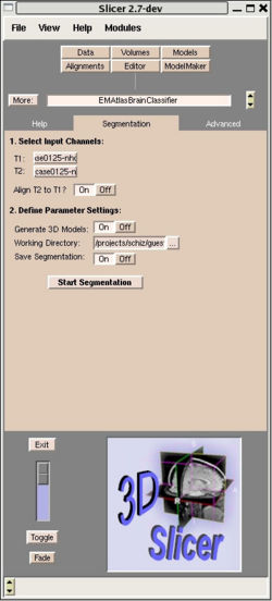
The EMAtlasBrainClassifier module basically implements the same expectation maximization algorithm as the Tcl script used in the current PNL processing pipeline. However, this module performs all four processing steps with a single button press. The user has to define the structural volume and the corresponding T2 volume and decides if step one (coregistration) is needed or not. Furthermore the user can turn on/off the output of various intermediate results of the segmentation algorithm under ”Advanced Tab”. Figure 1 shows a screenshot of the user interface of the EMAtlasBrainClassifier Module in Slicer.
An important feature is the possibility to toggle multi threading. Segmentation results were found to be dependent on the number of CPUs. This is due to the parallel implementation of the segmentation algorithm. To guarantee comparable results between computers with different numbers of CPUs, multithreading will be turned off in our new processing pipeline.
1.4 Motivation for the new pipeline
The new segmentation strategy only requires one click to initiate the process compared to four processing steps required by the old processing pipeline. Furthermore multithreading can be toggled with the Slicer module. The open source nature of 3DSlicer allows for the continuous integration of new, state-of-the art processing algorithms as well as the constant improvement of already existing modules. To assure the correctness of the EMSegmentation module output after a 3DSlicer update, we run an automated testing process comparing current module output to an expected module output for certain test cases.
The test result is automatically submitted to a webpage using the dashboard technology developed by Kitware.
2. Validation
2.1 Test cases
Seventy-eight cases of the PNL database for which the segmentation had already been created using the current pipeline were selected. We aimed to cover all disease databases in our lab in order to compare segmentation performance for all different disease-specific brain physiologies.
The following cases were selected:
| Database | Gender | Quantity |
|---|---|---|
| Chronic Schizophrenia | female | 2 |
| Chronic Schizophrenia | male | 10 |
| First Episode Schizophrenia | both | 10 |
| First Episode Schizophrenia, Brockton Studies (FEBS) | both | 10 |
| Schizotypal Personality Disorder (SPD) | female | 10 |
| Schizotypal Personality Disorder (SPD) | male | 10 |
| Velocardiofacial Syndrome (VCFS) | both | 4 |
| Normal Control: SPD | both | 8 |
| Normal Control: Chronic Schizophrenia | both | 10 |
| Normal Controls: First Episode Schizophrenia | both | 4 |
Quantities were chosen depending on the amount of cases we have within each database.
2.2 Measurements
By batch processing the EMAtlasBrainClassifier module in 3DSlicer, release 2.6, we generated the segmentation into gray matter, white matter, and CSF for each of the listed 78 cases. In order to compare old and new segmentation implementations the following measurements were calculated by a script written in Matlab:
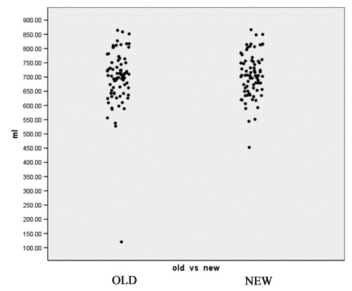
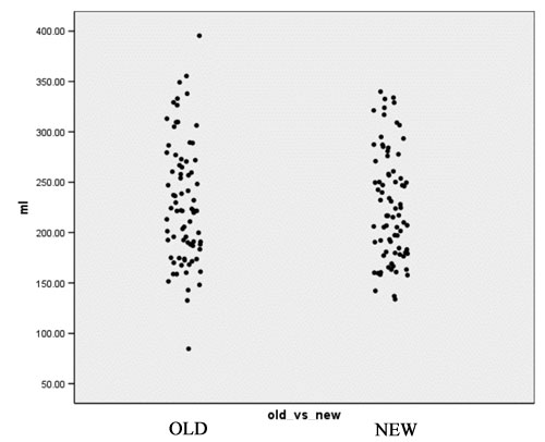
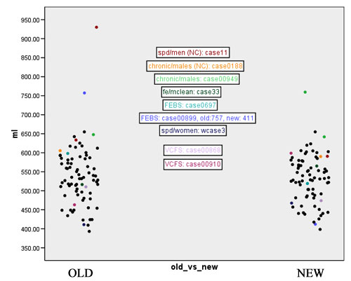
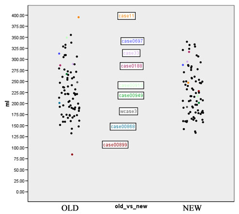
- Computation of volume for white matter, gray matter and CSF for every case for both the old and the new segmentation results. Figures 2 to 4 show the distributions of those tissue volumes in milliliter. The scatter plots for white matter, gray matter and CSF volume do not show any distribution differences between old and new segmentation results for any of those tissue classes.
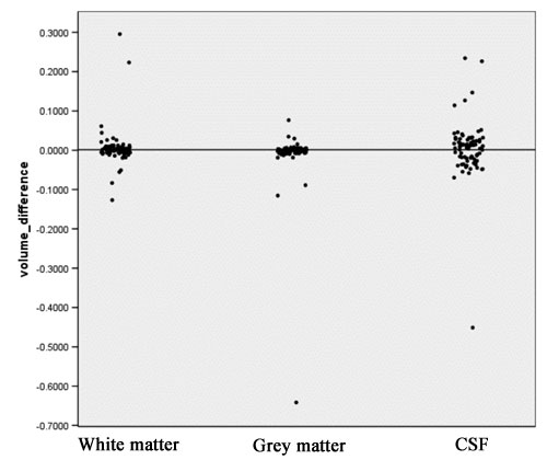
- Computation of volume differences for each tissue class, using the following equation:
  Vol_Diff = (V_1 – V_2)/(V_1 + V_2)
  V_1: Volume measured in the old segmentation result
  V_2: Volume measured in the new segmentation result
- This measure ranges from –1 to +1. When volume difference equals zero, exactly the same volume of this tissue class has been segmented for this case with both new and old methods. A negative value means more tissue was segmented by the new segmentation strategy compared to the old one.
- A positive volume difference means for this case more tissue was segmented by the old segmentation strategy.
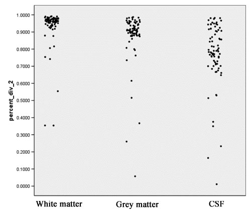
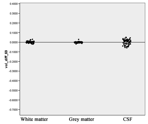
- The scatter plot in figure 5 visualizes the volume difference for white matter, gray matter, and CSF.
- Computation of the Jaccard Coefficient (also known as Dice) as a measure of overlap. For every tissue class both old and new segmentations are overlaid on top of each other. Intersection volume of both segmentations (V_1 AND V_2) and set union (V_1 OR V_2) are calculated for each tissue class.
- The Jaccard measure is defined by the equation:
JAC = (V_1 AND V_2) / (V_1 OR V_2)
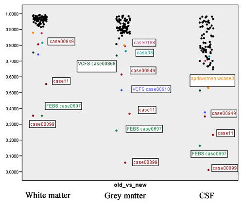
- Jaccard ranges from 0 (segmentations do not overlap at all) to +1 (segmentations completely agree). This measure is probably the most meaningful amongst those computed in the context of segmentation comparison. Figure 6 shows scatter plots for the Jaccard measure for white matter, grey matter and CSF.
- There are some cases where the Jaccard measure indicates that the segmentations do not overlap well. We had a closer look at those outliers.
2.3 Outliers
We selected all cases where the Jaccard measure for white matter was below 90% and defined those as outliers. A visual inspection yields a failure of the old segmentation method for 3 cases within those 9 outliers. This affects one case of a normal control located in the male SPD database and 2 cases in the FEBS database. For another 3 of those 9 outliers it turned out that the new segmentation method had failed. Those cases with an insufficient new segmentation result are located in the male chronic-schizophrenia database, the first-episode-schizophrenia database and the VCFS database. For the remaining 3 cases of the 9 outliers a visual inspection could not determine which segmentation is better or closer to the truth, respectively.
Figures 7 to 11 show again the scatter plots of white matter volume, gray matter volume, CSF volume, volume difference, and Jaccard measure, with the outliers marked. Both the volume differences plot (figure 10) and the Jaccard plot (figure 11) show the outliers result from the same 9 cases.
Volume differences and Jaccard measure distribution, with outliers removed, are shown in Figures 12 and 13.
2.4 Conclusion
- The volume distribution scatter plots show no difference between old and new method, suggesting that none of the two methods has a tendency to select more or less of any of the 3 tissue classes.
- The volume differences for white matter and gray matter are sufficiently close to 0, as can shown in Figure 12. The volume differences for CSF show more variability. This can be explained by a stronger dependency on the atlas registration which is the algorithm that underwent most changes in the new implementation.
- With the outliers removed, for all cases the white matter Jaccard measure is above 90% (that is how we defined outliers), for gray matter the Jaccard measure is above 80% for all non-outlier cases. Again, both segmentations agree the least for CSF determination as explained above.
Based on these observations and after discussion with Drs. Shenton and McCarley we decided to use the new method which is the EMSegmentation Module in 3DSlicer.
Assessing and comparing segmentation performance for different algorithm implementations is crucial to ensure reliable results for our neuroscience studies. Such an assessment and comparison should be performed for every future software change.
