Difference between revisions of "Projects:ProstateSegmentation"
| (38 intermediate revisions by 3 users not shown) | |||
| Line 1: | Line 1: | ||
| − | Back to [[Algorithm: | + | Back to [[Algorithm:Stony Brook|Stony Brook University Algorithms]] |
__NOTOC__ | __NOTOC__ | ||
= Prostate Segmentation = | = Prostate Segmentation = | ||
| − | The objective is to extract the prostate from a 3D ultrasound data set. | + | The objective is to extract the prostate from a 3D MRI and ultrasound data set. |
= Description = | = Description = | ||
| − | Two ways are employed to attack the problem. The first way is | + | Two ways are employed to attack the problem. The first way is Random Walks for prostate segmentation. While the second is using a shape based method. The details are given below. |
| + | Random Walks for prostate segmentation | ||
| − | == | + | == Overview == |
| − | + | The algorithm starts with a few initial seeds marking object and background. Then to decide the category of each of the other(non-seed) pixels, a random walker is released and it walks on the lattice of the image. The difficulty of walking from on pixel position to another is inversely related with the difference between the intensities of the two pixels. Given those settings, the probability of the random walker first hitting each kind of seeds are calculated. And the category of the pixel is assigned to the one with the greatest first hit probability. | |
| − | + | Ideally, through this process the category of each pixel in the image could be decided. | |
| − | + | == Algorithm detail == | |
| − | + | The philosophy of random walk segmentation being stated above, it's practically impossible to implement that way. (Say, releasing many random walkers at each pixel and get the first hit probability using Monte-Carlo method.) | |
| − | + | An analogy between first hit probability of random walks and the electrical potential distribution on a circuit network was given in the middle of last century. The resistance(conductance) in the circuit network is analogous to the crossing difficulty in the random walking scenario. Through the analogy the problem could be converted to a Dirichlet problem: | |
| + | <math> \triangle u = 0</math> | ||
| + | with boundary conditions: | ||
| + | <math>u = 1 for object seeds</math> | ||
| + | <math>u = 0 for background seeds</math> | ||
| − | + | In the above equation the <math>\triangle </math> is a Laplace-Beltrami operator where the spatial variant resistance is considered to be metric of the space. | |
| − | + | == Shape based segmentation == | |
| − | + | The shape based method could constrain the resulting segmentation within the learned variance of the shape. The algorithm consists two stages, learning the shapes and segment new case. | |
| − | == | + | == Shape learning == |
| − | + | The training set consists 29 data sets, each of which is manually segmented. Not only the prostate is segmented, but also the rectum. The reason for segmenting rectum will be given later. The segmented results are saved in label map where 0 indicates background, 1 means prostate while 2 is the rectum. | |
| − | + | To learn the shape of prostate, we first need to register them to get rid of the variance of rigid motion and isotropic scaling. | |
| − | This | + | There is very large shape variance in prostate. Just for ease of describing, we use ellipsoid analogy for the prostate. Some of the prostate has long axis horizontally posed, while some vertically. And some prostate is spherical shaped, having no eminent axis in any direction. So if we are to register the prostates alone, then the "horizontal prostate" would rotate 90 degree to best fit the "vertical prostate" and this may cause wrong point correspondence. This brings the necessity of having another object to "hold the frame", thus the rectum is also segmented out. |
| + | |||
| + | Having multiple objects to register at once, we employ the label space representation. It's a vectorial representation for multiple objects in image. Then a vector image registration process, based on the L-2 measure between two label space images, was carried on and 7 parameters(3 translation, 3 rotation and 1 isotropic scale) are registered. | ||
| + | |||
| + | Registration eliminates the similarity transform among shapes, next we learn the shape of prostate. The signed distance function(SDF) of the object has been used for shape learning by many researchers. In our case, we observed that two similar shapes may have large difference in the far field of their corresponding SDFs. However the shapes are embedded as the zero-contour of the SDF. So the large far field difference brings unnecessary variance. | ||
| + | |||
| + | To cure this, instead of learning SDFs, we learn the tanh(hyperbolic tangent) of SDF. The tanh function preserves the zero-contour of SDF while eliminates the far field variance. To sum up, we use tanh(SDF) to represent the shape. | ||
| + | |||
| + | Principle component analysis was carried on to learn the above representations of the shapes. And the eigen-vectors with high eigen-values are extracted as the basis of the shape space. Next, we segment a new image within this learned shape space, denoted as S. | ||
| + | |||
| + | == Segment new shape == | ||
| + | |||
| + | The new image to be segmented is first preprocessed to high light the region of prostate. Then, within the shape space S, we look for the one that after similarity transformation, best fits the preprocessed image. The fitness is defined by the Binomial energy proposed by Yezzi et. al. in ''A Statistical Approach to Snakes for Bimodal and Trimodal Imagery''. Next we detail the pre-processing and the segmentation. | ||
| + | |||
| + | == Pre-processing == | ||
| + | |||
| + | In the learning process we not only learn the shape, but also we could know the mean and standard divination of the intensity of prostate. For the given new image, we compute the likelihood image using the mean and std. To get the posterior image, uniform prior is used widely in literature. However that will include other regions with similar intensities. With another pieces of information, one point in the prostate, we could get better posterior image. That will further aid the segmentation. Next we detail the construction of prior. | ||
| + | |||
| + | Given one point in the prostate, preferred to be around center, we build a directional distance map. The local distances, from one grid point to its neighbors, are defined to be the absolute value of directional derivatives at that point toward its neighbors. By solving a Hamilton-Jacobi equation we obtain the directional distance map. The value of the distance map at each point illustrate both its Euclidean distance to the prostate and the similarity in intensity. | ||
| + | |||
| + | The prior is build by exp(-distance), and followed by the posterior map. In the later section, we'll call this posterior map by "distance modulated posterior map", or simply posterior map. | ||
| + | |||
| + | The posterior map given by uniform and distance modulated prior are, respectively: | ||
| + | |||
| + | [[Image:PosteriorWithUniformPrior.png|320px]] and [[Image:Posterior.png|320px]] | ||
| + | |||
| + | From which we can see that the distance modulated posterior eliminates the far field interference while maintain the shape(not favoring a spherical shape). | ||
| + | |||
| + | == Segmentation of the pre-processed image == | ||
| + | |||
| + | Given the posterior map, we want to find one shape in the shape space to minimize the Binomial energy. Because the shape in the learned shape space is represented by basis, instead of evolving the curve/surface, we only need to optimize over the coefficients of the basis. So the problem is turned into a finite dimensional non-linear optimization problem. | ||
| + | |||
| + | We calculate the gradient of the energy with respect to shape basis coefficients and similarity transformation parameters. Then we use the non-linear optimization algorithm LBFGS to get the result, shown in | ||
| + | |||
| + | [[Image:ShapeBasePstSegSlicer.png|Shape base prostate segmentation in Slicer through command line module|500px]]. | ||
| + | |||
| + | As shown in the above image, the algorithm is integrated into 3D Slicer. | ||
= Key Investigators = | = Key Investigators = | ||
| Line 41: | Line 82: | ||
= Publications = | = Publications = | ||
| + | In Press | ||
| + | |||
| + | Y. Gao, R. Sandhu, G. Fichtinger, A. Tannenbaum; A coupled global registration and segmentation framework with application to magnetic resonance prostate imagery. IEEE TMI (in submission) | ||
| + | |||
| + | = Recent Work = | ||
| + | [[RobustStatisticsSegmentation| Robust Statistics Segmentation]] | ||
| + | Project Week Results: [[2009_Summer_project_week_prostate_registration|Jun 2009]] | ||
| − | [[Category: Segmentation]] | + | [[Category: Segmentation]] [[Category: Prostate]] |
Latest revision as of 01:00, 16 November 2013
Home < Projects:ProstateSegmentationBack to Stony Brook University Algorithms
Prostate Segmentation
The objective is to extract the prostate from a 3D MRI and ultrasound data set.
Description
Two ways are employed to attack the problem. The first way is Random Walks for prostate segmentation. While the second is using a shape based method. The details are given below.
Random Walks for prostate segmentation
Overview
The algorithm starts with a few initial seeds marking object and background. Then to decide the category of each of the other(non-seed) pixels, a random walker is released and it walks on the lattice of the image. The difficulty of walking from on pixel position to another is inversely related with the difference between the intensities of the two pixels. Given those settings, the probability of the random walker first hitting each kind of seeds are calculated. And the category of the pixel is assigned to the one with the greatest first hit probability.
Ideally, through this process the category of each pixel in the image could be decided.
Algorithm detail
The philosophy of random walk segmentation being stated above, it's practically impossible to implement that way. (Say, releasing many random walkers at each pixel and get the first hit probability using Monte-Carlo method.)
An analogy between first hit probability of random walks and the electrical potential distribution on a circuit network was given in the middle of last century. The resistance(conductance) in the circuit network is analogous to the crossing difficulty in the random walking scenario. Through the analogy the problem could be converted to a Dirichlet problem: [math] \triangle u = 0[/math] with boundary conditions: [math]u = 1 for object seeds[/math] [math]u = 0 for background seeds[/math]
In the above equation the [math]\triangle [/math] is a Laplace-Beltrami operator where the spatial variant resistance is considered to be metric of the space.
Shape based segmentation
The shape based method could constrain the resulting segmentation within the learned variance of the shape. The algorithm consists two stages, learning the shapes and segment new case.
Shape learning
The training set consists 29 data sets, each of which is manually segmented. Not only the prostate is segmented, but also the rectum. The reason for segmenting rectum will be given later. The segmented results are saved in label map where 0 indicates background, 1 means prostate while 2 is the rectum.
To learn the shape of prostate, we first need to register them to get rid of the variance of rigid motion and isotropic scaling.
There is very large shape variance in prostate. Just for ease of describing, we use ellipsoid analogy for the prostate. Some of the prostate has long axis horizontally posed, while some vertically. And some prostate is spherical shaped, having no eminent axis in any direction. So if we are to register the prostates alone, then the "horizontal prostate" would rotate 90 degree to best fit the "vertical prostate" and this may cause wrong point correspondence. This brings the necessity of having another object to "hold the frame", thus the rectum is also segmented out.
Having multiple objects to register at once, we employ the label space representation. It's a vectorial representation for multiple objects in image. Then a vector image registration process, based on the L-2 measure between two label space images, was carried on and 7 parameters(3 translation, 3 rotation and 1 isotropic scale) are registered.
Registration eliminates the similarity transform among shapes, next we learn the shape of prostate. The signed distance function(SDF) of the object has been used for shape learning by many researchers. In our case, we observed that two similar shapes may have large difference in the far field of their corresponding SDFs. However the shapes are embedded as the zero-contour of the SDF. So the large far field difference brings unnecessary variance.
To cure this, instead of learning SDFs, we learn the tanh(hyperbolic tangent) of SDF. The tanh function preserves the zero-contour of SDF while eliminates the far field variance. To sum up, we use tanh(SDF) to represent the shape.
Principle component analysis was carried on to learn the above representations of the shapes. And the eigen-vectors with high eigen-values are extracted as the basis of the shape space. Next, we segment a new image within this learned shape space, denoted as S.
Segment new shape
The new image to be segmented is first preprocessed to high light the region of prostate. Then, within the shape space S, we look for the one that after similarity transformation, best fits the preprocessed image. The fitness is defined by the Binomial energy proposed by Yezzi et. al. in A Statistical Approach to Snakes for Bimodal and Trimodal Imagery. Next we detail the pre-processing and the segmentation.
Pre-processing
In the learning process we not only learn the shape, but also we could know the mean and standard divination of the intensity of prostate. For the given new image, we compute the likelihood image using the mean and std. To get the posterior image, uniform prior is used widely in literature. However that will include other regions with similar intensities. With another pieces of information, one point in the prostate, we could get better posterior image. That will further aid the segmentation. Next we detail the construction of prior.
Given one point in the prostate, preferred to be around center, we build a directional distance map. The local distances, from one grid point to its neighbors, are defined to be the absolute value of directional derivatives at that point toward its neighbors. By solving a Hamilton-Jacobi equation we obtain the directional distance map. The value of the distance map at each point illustrate both its Euclidean distance to the prostate and the similarity in intensity.
The prior is build by exp(-distance), and followed by the posterior map. In the later section, we'll call this posterior map by "distance modulated posterior map", or simply posterior map.
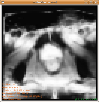
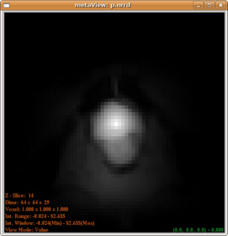
The posterior map given by uniform and distance modulated prior are, respectively:
From which we can see that the distance modulated posterior eliminates the far field interference while maintain the shape(not favoring a spherical shape).
Segmentation of the pre-processed image
Given the posterior map, we want to find one shape in the shape space to minimize the Binomial energy. Because the shape in the learned shape space is represented by basis, instead of evolving the curve/surface, we only need to optimize over the coefficients of the basis. So the problem is turned into a finite dimensional non-linear optimization problem.
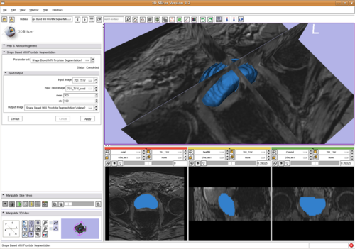
We calculate the gradient of the energy with respect to shape basis coefficients and similarity transformation parameters. Then we use the non-linear optimization algorithm LBFGS to get the result, shown in
As shown in the above image, the algorithm is integrated into 3D Slicer.
Key Investigators
- Georgia Tech Algorithms: Yi Gao, Allen Tannenbaum
Publications
In Press
Y. Gao, R. Sandhu, G. Fichtinger, A. Tannenbaum; A coupled global registration and segmentation framework with application to magnetic resonance prostate imagery. IEEE TMI (in submission)
Recent Work
Robust Statistics Segmentation
Project Week Results: Jun 2009


