Projects:LongitudinalShapeAnalysis
Back to Utah 2 Algorithms
Ongoing Work
Analysis of Longitudinal Shape Variability
Quantification of anatomical variability within a population and between populations are fundamental tasks in medical imaging studies. In many clinical applications, it is particularly crucial to quantify anatomical variability over time in order to determine disease progression and to isolate clinically important differences in both space and time. Such studies are designed around longitudinal imaging, where we acquire repeated measurements over time of the same subject, which yields rich data for analysis. Statistical analysis of longitudinal anatomical data is a problem with significant challenges due to the difficulty in modeling anatomical changes, such as growth, and comparing changes across different populations.
In this project, we propose a new approach for analyzing statistical variability of shapes over time, in the spirit of which is based on combining cross-sectional atlas construction with subject specific growth modeling. The growth model used for shape regression naturally handles multiple shapes at each time point and does not require point correspondence between subjects, making the proposed framework both convenient and applicable to a wide range of clinical problems.
Description
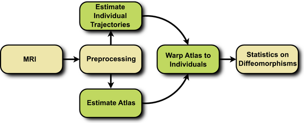
The proposed framework consists of three steps, summarized in Fig. 1. First, a cross-sectional atlas is estimated by shape regression, which can be thought of Fig. 1. Flowchart depicting the proposed method. as normative, reference evolution. Second, subject specific growth trajectories are estimated independently for each individual, accounting for intra-subject variability. Third, a homologous space for statistical analysis is obtained by warping the atlas to each individual at any time point of interest.
The first two steps require the estimation of a growth model, the specifics of which are discussed in the next section. Here we use the acceleration controlled growth model of [1], where shape evolution is modeled as a continuous flow of deformation. A baseline shape is continuously deformed over time to match the target shapes. The estimation is posed as a variational problem balancing fidelity to data with regularity.
The parameterization by acceleration guarantees that the estimated evolution is temporally smooth. Furthermore, the acceleration controlled growth model is generic, with no constraint that the flow of deformation must follow a geodesic path, or close to a geodesic path. For measuring shape similarity, we use the metric on currents [2]. This way, shapes are modeled as distributions, alleviating the need for explicit point correspondence between shapes.
We extract shape features, which are diffeomorphisms that map the reference atlas to each subject at a specific time point. This is accomplished by warping the atlas to each subject at the time point of interest using the registration framework of [10]. Due to regression, we can construct a shape from the atlas and from any individual at any time of interest. The warping from atlas space to each individual establishes homologous points between every subject.
The flow of diffeomorphisms that warp the template shape to each individual subject shape are geodesic [3]. As a result, the initial momenta completely determine the entire deformation. Since the atlas is warped to each subject, every diffeomorphism starts from the same reference space. We can leverage this common vector space to compute intrinsic statistics. For example, a mean can be computed by simply taking the arithmetic mean of a collection of momenta fields. The mean momenta can then be applied to a shape via geodesic shooting.
Results
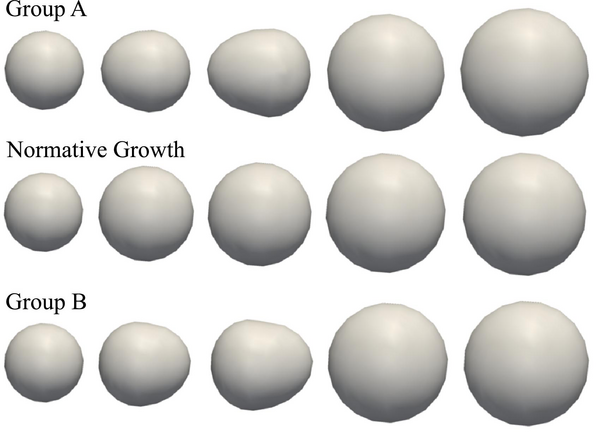
Synthetic Data We first evaluate our framework with a database of synthetic longitudinal shape data. In this simple database, normative growth is modeled by a sphere which grows isotropically over time. We further consider two groups, A and B, with different patterns of growth. Group A starts as a small sphere, develops a protuberance in the negative x direction, and eventually evolves into large sphere. Group B also starts from a small sphere, but develops a protuberance in the positive x direction, before evolving into a large sphere. Subjects from both groups contain 5 time points corresponding to 6, 10, 12, 18, and 24 months. We construct 12 subjects in each group by randomizing the amount of protuberance and also the amount of global scaling. A typical subject from group A and group B as well as the normative reference growth are summarized in Fig 2.
First, we perform PCA on the momenta that warp the normative atlas to each individual in group A. The first major mode of variation is summarized in Fig. 3 for several time points. This mode explains the variability in group A with respect to the reference shapes. The bulge on the left side of the shape is clearly identified along with variability in scale. A PCA on group B produces similar results, however it captures the bulge on the right side of the shape.
We also conduct hypothesis testing to determine if there are significant differences between group A and B. For each shape point, an independent t-test is performed on the magnitude of initial momenta which parameterize the mapping from reference atlas to individuals. We are testing if the distribution of momenta magnitude at each shape point is different between each group. Fig. 4 shows the Bonferroni corrected p-values shown on the reference atlas at selected time points. We observe significance on the left and right side of the shapes at 9, 12, and 16 months, corresponding to the bulge growing in opposite directions in group A and B. It is also important to note that we observe no significant differences at 20 months, where the shapes of each group are nearly identical.
Clinical Data We also evaluate our method using a longitudinal database from an Autism Center of Excellence, part of the Infant Brain Imaging Study (IBIS). The study consists of high-risk infants as well as controls, scanned at approximately 6, 12, and 24 months. At 24 months, symptoms of autism spectrum disorder (ASD) were measured using the Autism Diagnostic Observation Schedule (ADOS). A positive ADOS score indicates the child has a high probability of later being diagnosed with autism. Finally, we have three groups: 15 high-risk subjects with positive ADOS (HR+), 40 high-risk subjects with negative ADOS (HR-), and 14 low-risk subjects with negative ADOS (LR-).
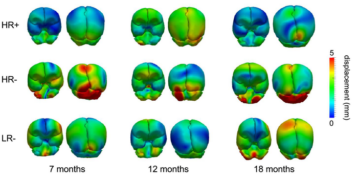
We investigate the shape variability in the HR+ and HR- groups by performing PCA on the initial momenta for each group. Recall that PCA is conducted using the momenta vectors that parameterize the mapping from atlas to subject at each selected time point. Therefore, the major modes of variability describe how each group varies from the normative growth scenario, shown in Fig. 5 for several time points of interest. There appears to be a difference in how each group deviates from the normative growth scenario, particularly in the cerebellum. This could be an interesting avenue to pursue for future research.
Hypothesis testing is conducted on the magnitude of initial momenta between groups. For each shape point, we perform a t-test on the distribution of momenta magnitude between each population. After correcting the p-value for multiple comparisons, using Bonferroni correction, we find no significant locations on the surfaces of the left/right hemisphere or cerebellum. This may be due to relatively small sample size. However, it may be the case that smaller scale anatomical surfaces, such as subcortical structures might lead to group discrimination due to hypothesized differences in brain growth.
It is important to stress that these results are intended to illustrate a potential application of our methodology. The results here are too preliminary to draw meaningful conclusions with respect to autism, due to the small sample size and the need to incorporate biostatistical modeling, that combines patient variables with our computational analysis.
Literature
[1] Fishbaugh, J., Durrleman, S., Gerig, G.: Estimation of smooth growth trajectories with controlled acceleration from time series shape data. In: Fichtinger, G., Peters, T. (eds.) MICCAI. LNCS, vol. 6892, pp. 401–408. Springer (2011)
[2] Vaillant, M., Glaunes, J.: Surface matching via currents. In: IPMI. LNCS, vol. 3565, pp. 381–392. Springer (2005)
[3] Miller, M, I., Trouve, A., Younes, L.: On the metrics and Euler-Lagrange equations of Computational Anatomy. Annual Review of Biomedical Engineering 4, 375–405 (2002)
[4] Muralidharan, P., Fishbaugh, J., Johnson, H., Durrleman, S., Paulsen, J., Gerig, G., Fletcher, P.T. Diffeomorphic shape trajectories for improved longitudinal segmentation and statistics. Proc. of Medical Image Computing and Computer Assisted Intervention (MICCAI '14). (2014).
Key Investigators
- Utah: James Fishbaugh, Marcel Prastawa, Guido Gerig
- INRIA/ICM, Pitie Salpetriere Hospital: Stanley Durrleman
- Carolina Institute for Developmental Disabilities: Joseph Piven


