Projects:RegistrationDocumentation:RegEval Anisotropy
Effects of Voxel Anisotropy and Intensity-Inhomogeneity on Image-based 3D Registration
Dominik Meier, William Wells III, Andriy Fedorov, C.F. Westin, Ron Kikinis
Summary / Questions
This is a planned experiment & manuscript for results/models on how voxel-anisotropy and MR bias fields affect automated, intensity-based image registration, mostly in terms of precision and robustness. Given the complexity of interaction between cost function, optimizer & input data, much of the experiments will likely be empirical evidence, but other (theoretical/analytical) exploits would be welcome. Chief questions are:
- Anisotropy
- at what point does voxel anisotropy seriously affect registration performance?
- are individual DOF affected in different ways, i.e. how much more sensitive is rotation to this effect than other DOF?
- what are the remedies & recommendations, e.g. images with voxel anisotropy ratios above X should be resampled or traverse DOF space in different ways (e.g. does isolate/constrain the most sensitive DOF help)?
- strategies for non-rigid registration
- Intensity-Inhomogeneity
- does bias field inhomogeneity in MRI images affect the quality of automated registration?
- What is the relative sensitivity of different cost functions (MI vs. NormCorr)?
- Is there a level where the bias field begins to compete with image content?
- Should a bias-field correction be applied beforehand or after? Is bias correction affected by prior registration?
- what is the effect of "differential bias"? for the purpose of subtraction and/or ratio images, is differential bias correction (Lewis et al. NeuroImage 2004) preferable to correcting each bias individually? Determined as residual in validation images of zero or predefined diff. -> moving out of scope a bit, because it is no longer pure registration but includes change detection via subtraction. On the other hand that is the common application and hence clarity on bias sources is needed. Most common applications for intra-subject intra-modality registration is are change detection, image guidance & image fusion.
Methods
The basic experiment proposed is to take reference images with high-resolution and isotropic voxel size; move them by a known amount, then filter & subsample to simulate anisotropy; and finally register & evaluate residual error. The self-validation format is there because having a ground truth is the easiest way to isolate the effects under study, but roughly any image pair with an acceptable gold-standard alignment is eligible. More detailed analyses of cost function behavior, capture range etc. are also possible.
- Test Data
- isotropic resolution required, 1mm or small enough to allow subsampling by factors 2-3 and still remain in range of clinically relevant settings
- organs: brain, kidney, breast,
- modalities: MRI (incl. DTI, fMRI), CT
- Brainweb
- modalities where anisotropy is common AF: use case: anisotropy is common in diagnostic T2w prostate MRI, typical resolution is ~0.5x0.5x3 mm
- Anisotropy Experiment
- take 1mm iso ref volume and move by known amount
- filter (1-D avg filter) & subsample both image grids
- register & evaluate residual error (evaluate RMS distance: distance of ICC points sent through R1*inv(R2)
- we would like to isolate as best as possible the anisotropy effect from correlates such as overall resolution etc. Hence it seems appropriate to match the two image pairs being compared in voxel volume, e.g. the isotropic reference for a 1x1x3 mm image would be 1.44mm isotropic (3^.333), so that we can argue the two images contain (from a "volumetric" viewpoint) the same amount of information.
- proper subsampling: Since the resampler performs a backward mapping and we cannot control the parameters like the sinc window, we should run a linear avg. filter over the volume to simulate the PV effect before subsampling. E.g. a 1.5 anisotropy would be convolving with a 2x1 kernel [2 1]/3 , a 3.0 anisotropy would be a [1 1 1]/3 kernel etc. Simplest to convolve once each axis separately. Implementation options: Pyhton -> ITK, Compiled Matlab
- BiasField Experiment:
- take 1mm iso ref volume and move by known amount
- apply bias field to both image grids
- register & evaluate residual error
- Variational Parameters
- voxel size factors: x 1 , 1.2 , 1.5 , 3 , 5, 10
- bias field: derive from actual case, then amplify x 1 , 1.2 , 1.5
- reference motion
- registration sampling rate
- to obtain Relevant Reference XForm: take 2 real-life scans of different protocols, e.g. FLAIR and T1, and perform BSpline registration, use that as reference + add additional translation & rotation
- Evaluation
- registration error as RMS residual
- cost function
- ROC?
Literature
- Bias Correction + Registration (SPIE 2003)
- Evaluation of BSpline Registration Error(TMI 2009)
- Differential Bias Correction (NeuroImage 2004)
- Importance Sampling for Nonrigid Registr (TMI 2009)
- Automated Parameter Selection (TMI 2010)
Timeframe
- body of results by registration retreat in February 2011?
- manuscript submitssion around April 2011?
Experiment 1: Anisotropy degenerates Joint Histogram & Global Optimum
- Rationale: This experiment produces directly joint histograms and difference(ratio) images w/o the need to run the actual registration, i.e. we compare the effects of voxel anisotropy on the theoretical optimum: Move, filter and subsample identical image pair, then resample back to original position and build joint histograms and subtraction images. Because of the increasing PV effects we expect to see a degenerating joint histogram and a subtraction image with increasing edge artifacts. We can then try to interpret how the optimizer will behave in this environment. The benefit of this metric is that we circumvent the stochastic nature of the registration output.
- Pipeline
- original
- move by known amount (Aff0)
- PV filter blur + subsample to anisotropic voxel size
- rotate back (inv(Aff0))
- upsample to original size
- compute joint histogram
- evaluate relative blurring: deviation from unity line
- Results
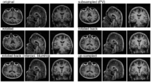
Fig.1: Example processing pipeline simulating PV effects from anisotropic voxel size
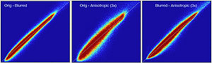
Fig.2: Example joint histogram. left: reference blurring from interpolation blurring alone (no PV); middle: 3x1 anisotropy against original; right: 3:1 anisotropy against blurred reference

Fig.3: same as Fig.2 for anisotropy ratio 5:1
Fig.4: Example joint histogram blurring effects from anisotropic voxel size : 1x to 20x anisotropy
Fig.5: for comparison: example joint histogram blurring effects from rotation around x (LR) axis 1-15 degrees
Fig.6: for comparison: example joint histogram blurring effects from rotation around y (AP) axis 1-15 degrees

Fig.7: for comparison: example joint histogram blurring effects from rotation around z (IS) axis 1-15 degrees
Fig.8: for comparison: example joint histogram blurring effects from translation only along x (LR) axis 1-15 pixels


- Discussion
- need an intuitive way or metric to interpret the blurring of the JH, what it means in terms of registration accuracy, robustness, capture range etc. One way would be to quantify the off-diagnoal amount of intensity, another more visual to compare to blurring from misalignment, i.e. find the misalignment that produces a similarly blurred JH.
- the blurred histogram represents the new practically achievable global optimum, relative to the theoretical ideal of a 45-degree unity line
- the partial volume "bleed" works relative to the histogram mode/mean, i.e. low intensities are more likely to get brighter by PV, whereas higher intensities are more likely to be surrounded by lower ones and hence become darker by PV. Thus the joint histogram gets "squished" toward the middle from both ends (Fig.1), and ends up with a rotation relative to the 45 axis around a midpoint that's somewhere near the mode or mean intensity. We could measure this rotation as another metric. Most straightforward would be via principal axes.
- we have a mix between many points with small distances from the axis, and few points with large distances, hence the original histogram appears "mixed in" in a summary of off-diagnoal energy. How to calibrate the two is best answered by how the registration algorithm evaluates the joint histogram shape into its cost function.
- blurring for reference rotations and translations looks largely the same, so we use translation for ease of use (clearly defined residual RMS)
- measuring off-diagnoal energy: Mattes MI as implemented in ITK: extract code & compute as standalone
Experiment 2: Anisotropy most strongly affects rotation axes perpendicular to the largest voxel dimension
- Rationale: we assume registration is more likely to fail for anisotropic voxels because 1) there is less edge information that is critical in matching accuracy, 2) the optimization landscape is less smooth, increasing the likelihood for the optimizer to get stuck in local minima. Further we expect strongest sensitivity when to rotation axes are perpendicular to the largest voxel dimension; e.g. if we have 1x1x3mm axial slices, rotations around the z-axis (i.e. in plane) are far less critical than rotations around x- or y-axes. Similarly if largest voxel direction is not along dominant image content/object we have larger partial volume effects. E.g. for brain MRI most of the basal ganglia have a dominant C-shape that is best represented in coronal slices, and hence would be least sensitive to anisotropy in AP-direction.
- Capture Range is a parameter suitable for evaluating optimizer-related effects; it describes a region of parameter space around a (global) optimum where the solution converges to that optimum. We would therefore expect a reduced capture range if the optimizer is affected, i.e. if the anisotropy destroys the smoothness of the optimization landscape, this is expressed i a reduction of the capture range.
- Variation parameters:
- anisotropy ratios 1.2, 1.5, 2, 3, 5, 10: we build 2 image pairs each with the same misalignment/pose to be recovered; one image pair is anisotropic, the other isotropic of equivalent volume.
- rotation axis: LR, AP, IS
- rotation amount: 2,5,10,15,20,25,30 degrees
- Variant 1: we fix the axis and run the full 2D landscape of anisotropy and rotation angle
- Variant 2: we first run a pilot with the full isotropic images where we find the rotation failure point as indicator of capture range: increase rotation until we reach a failure point. We then repeat this for increasing anisotropy and compare the failure point limit. This would seem to promise less stochastic results that are easier to interpret.